Detrended Fluctuation Analysis (DFA)

fd_dfa

fd_dfa(
  y,
  fs = NULL,
  removeTrend = c("no", "poly", "adaptive", "bridge")[2],
  polyOrder = 1,
  standardise = c("none", "mean.sd", "median.mad")[2],
  adjustSumOrder = FALSE,
  removeTrendSegment = c("no", "poly", "adaptive", "bridge")[2],
  polyOrderSegment = 1,
  scaleMin = 4,
  scaleMax = stats::nextn(floor(NROW(y)/2), factors = 2),
  scaleResolution = log2(scaleMax) - log2(scaleMin),
  dataMin = NA,
  scaleS = NA,
  overlap = NA,
  doPlot = FALSE,
  returnPlot = FALSE,
  returnPLAW = FALSE,
  returnInfo = FALSE,
  silent = FALSE,
  noTitle = FALSE,
  tsName = "y"
)

Arguments

y: A numeric vector or time series object.
fs: Sample rate
removeTrend: Method to use for global detrending (default = "poly")
polyOrder: Order of global polynomial trend to remove if removeTrend = "poly". If removeTrend = "adaptive" polynomials 1 to polyOrder will be evaluated and the best fitting curve (R squared) will be removed (default = 1)
standardise: Standardise the series using ts_standardise() with adjustN = FALSE (default = "mean.sd")
adjustSumOrder: Adjust the time series (summation or difference), based on the global scaling exponent, see e.g. Ihlen (2012) (default = FALSE)
removeTrendSegment: Method to use for detrending in the bins (default = "poly")
polyOrderSegment: The DFA order, the order of polynomial trend to remove from the bin if removeTrendSegment = "poly". If removeTrendSegment = "adaptive" polynomials 1 to polyOrder will be evaluated and the best fitting polynomial (R squared) will be removed (default = 1)
scaleMin: Minimum scale (in data points) to use for log-log regression (default = 4)
scaleMax: Maximum scale (in data points) to use for log-log regression. This value will be ignored if dataMin is not NA, in which case bins of size < dataMin will be removed (default = stats::nextn(floor(NROW(y)/4), factors = 2))
scaleResolution: The scales at which detrended fluctuation will be evaluated are calculated as: seq(scaleMin, scaleMax, length.out = scaleResolution) (default = round(log2(scaleMax-scaleMin))). #' @param dataMin Minimum number of data points in a bin required for inclusion in calculation of the scaling relation. For example if length(y) = 1024 and dataMin = 4, the maximum scale used to calculate the slope will be 1024 / 4 = 256. This value will take precedence over the scaleMax (default = NA)
scaleS: If not NA, it should be a numeric vector listing the scales on which to evaluate the detrended fluctuations. Arguments scaleMax, scaleMin, scaleResolution and dataMin will be ignored (default = NA)
overlap: A number in [0 ... 1] representing the amount of 'bin overlap' when calculating the fluctuation. This reduces impact of arbitrary time series begin and end points. If length(y) = 1024 and overlap is .5, a scale of 4 will be considered a sliding window of size 4 with step-size floor(.5 * 4) = 2, so for scale 128 step-size will be 64 (default = NA)
doPlot: Output the log-log scale versus fluctuation plot with linear fit by calling function plotFD_loglog() (default = TRUE)
returnPlot: Return ggplot2 object (default = FALSE)
returnPLAW: Return the power law data (default = FALSE)
returnInfo: Return all the data used in SDA (default = FALSE)
silent: Silent-ish mode (default = FALSE)
noTitle: Do not generate a title (only the subtitle) (default = FALSE)
tsName: Name of y added as a subtitle to the plot (default = "y")

Value

Estimate of Hurst exponent (slope of log(bin) vs. log(RMSE)) and an FD estimate based on Hasselman (2013) A list object containing:

A data matrix PLAW with columns freq.norm, size and bulk.
Estimate of scaling exponent sap based on a fit over the standard range (fullRange), or on a user defined range fitRange.
Estimate of the the Fractal Dimension (FD) using conversion formula's reported in Hasselman(2013).
Information output by various functions.

References

Hasselman, F. (2013). When the blind curve is finite: dimension estimation and model inference based on empirical waveforms. Frontiers in Physiology, 4, 75. https://doi.org/10.3389/fphys.2013.00075

Author

Fred Hasselman

Examples


set.seed(1234)

# Brownian noise
fd_dfa(cumsum(rnorm(512)))
#> 
#> 
#> (mf)dfa:	Sample rate was set to 1.
#> 
#> 
#> ~~~o~~o~~casnet~~o~~o~~~
#> 
#>  Detrended Fluctuation Analysis 
#> 
#>  Full range (n = 7)
#> Slope = 1.46 | FD = 1.08 
#> 
#>  Exclude large bin sizes (n = 6)
#> Slope = 1.51 | FD = 1.07 
#> 
#>  Detrending: poly
#> 
#> ~~~o~~o~~casnet~~o~~o~~~

# Brownian noise with overlapping bins
fd_dfa(cumsum(rnorm(512)), overlap = 0.5)
#> 
#> 
#> (mf)dfa:	Sample rate was set to 1.
#> 
#> 
#> ~~~o~~o~~casnet~~o~~o~~~
#> 
#>  Detrended Fluctuation Analysis 
#> 
#>  Full range (n = 7)
#> Slope = 1.49 | FD = 1.07 
#> 
#>  Exclude large bin sizes (n = 7)
#> Slope = 1.49 | FD = 1.07 
#> 
#>  Detrending: poly
#> 
#> ~~~o~~o~~casnet~~o~~o~~~

# Brownian noise to white noise - windowed analysis
y <- rnorm(1024)
y[1:512] <- cumsum(y[1:512])

id <- ts_windower(y, win = 256, step = 1)

DFAseries <- plyr::ldply(id, function(w){
fd <- fd_dfa(y[w], silent = TRUE)
return(fd$fitRange$FD)
})

op <- par(mfrow=c(2,1))
plot(ts(y))
plot(ts(DFAseries[,2]))
lines(c(0,770),c(1.5,1.5), col = "red3")
lines(c(0,770),c(1.1,1.1), col = "steelblue")

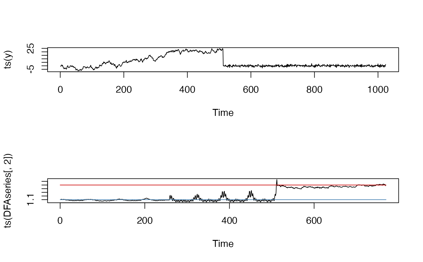par(op)