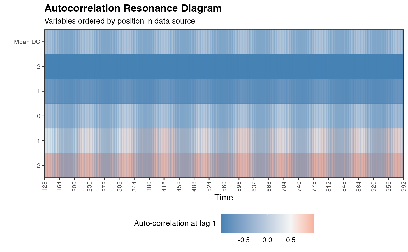
Calculate the autocorrelation function in a right-aligned sliding window on (multivariate) time series data.
Usage
ac_win(
  df,
  win = NROW(df),
  doPlot = FALSE,
  useVarNames = TRUE,
  colOrder = TRUE,
  useTimeVector = NA,
  timeStamp = "31-01-1999"
)
Arguments
- df
A data frame containing multivariate time series data from 1 person. Rows should indicate time, columns should indicate the time series variables. All time series in
dfshould be on the same scale, an error will be thrown if the range of the time series indfis not[scale_min,scale_max].- win
Size of window in which to calculate Dynamic Complexity. If
win < NROW(df)the window will move along the time series with a stepsize of1(default =NROW(df))- doPlot
If
TRUEshows a Complexity Resonance Diagram of the Dynamic Complexity and returns an invisibleggplot2::ggplot()object. (default =FALSE)- useVarNames
Use the column names of
dfas variable names in the Complexity Resonance Diagram (default =TRUE)- colOrder
If
TRUE, the order of the columns indfdetermines the of variables on the y-axis. UseFALSEfor alphabetic/numeric order. UseNAto sort by by mean value of Dynamic Complexity (default =TRUE)- useTimeVector
Parameter used for plotting. A vector of length
NROW(df), containing date/time information (default =NA)- timeStamp
If
useTimeVectoris notNA, a character string that can be passed tolubridate::stamp()to format the the dates/times passed inuseTimeVector(default ="01-01-1999")
Note
For different step-sizes or window alignments see ts_windower().
Examples
data(ColouredNoise)
ac_win(elascer(ColouredNoise[,c(1,11,21,31,41)],groupwise = TRUE), win = 128, doPlot = TRUE)
#> Warning: Using `size` aesthetic for lines was deprecated in ggplot2 3.4.0.
#> ℹ Please use `linewidth` instead.
#> ℹ The deprecated feature was likely used in the casnet package.
#>   Please report the issue at <https://github.com/FredHasselman/casnet/issues>.
#> Warning: Removed 960 rows containing missing values or values outside the scale range
#> (`geom_raster()`).
#> Warning: Removed 31 rows containing missing values or values outside the scale range
#> (`geom_vline()`).