Using the CRQA command line interface (rp_cl)
Fred Hasselman
2019-10-07
Source:vignettes/cl_RQA.Rmd
cl_RQA.RmdAn R interface to Marwan’s commandline recurrence plots
The rp_cl() function is a wrapper for the executables provided by Norbert Marwan.
The rp executable is installed when the function is called for the first time:
- It is renamed to
rpfrom a platform specific filename located in the directory: [path to casnet]/commandline_rp/ - The file is copied to the directory: [path to casnet]/exec/
- The latter location is stored as an option and can be read by calling
getOption("casnet.path_to_rp")
Note that the platform specific rp command line executables were created by Norbert Marwan and obtained under a Creative Commons License from the website of the Potsdam Institute for Climate Impact Research at: http://tocsy.pik-potsdam.de/
The full copyright statement on the website is as follows:
© 2004-2017 SOME RIGHTS RESERVED
University of Potsdam, Interdisciplinary Center for Dynamics of Complex Systems, Germany
Potsdam Institute for Climate Impact Research, Transdisciplinary Concepts and Methods, Germany
This work is licensed under a Creative Commons Attribution-NonCommercial-NoDerivs 2.0 Germany License.
More information about recurrence quantification analysis can be found on the Recurrence Plot website.
Auto RQA
We’ll use data from Oomens, Maes, Hasselman, & Egger (2015) in which 242 students were asked to generate random sequences of 100 numbers between 1 and 9 (for details see the article).
library(casnet)
library(ggplot2)

# Load the random number sequence data from Oomens et al. (2015)
data(RNG)

# Select a subject
IDs <- RNG$ID%in%c(163,291)

# Look at the sequence
ggplot(RNG[IDs,],aes(x=time,y=number,group=ID)) +
  geom_line(aes(colour=ID))+
  facet_grid(~ID) +
  scale_y_continuous(breaks = 1:9) +
  ggtitle("Which of these number sequences is more 'random'?") +
  theme_bw()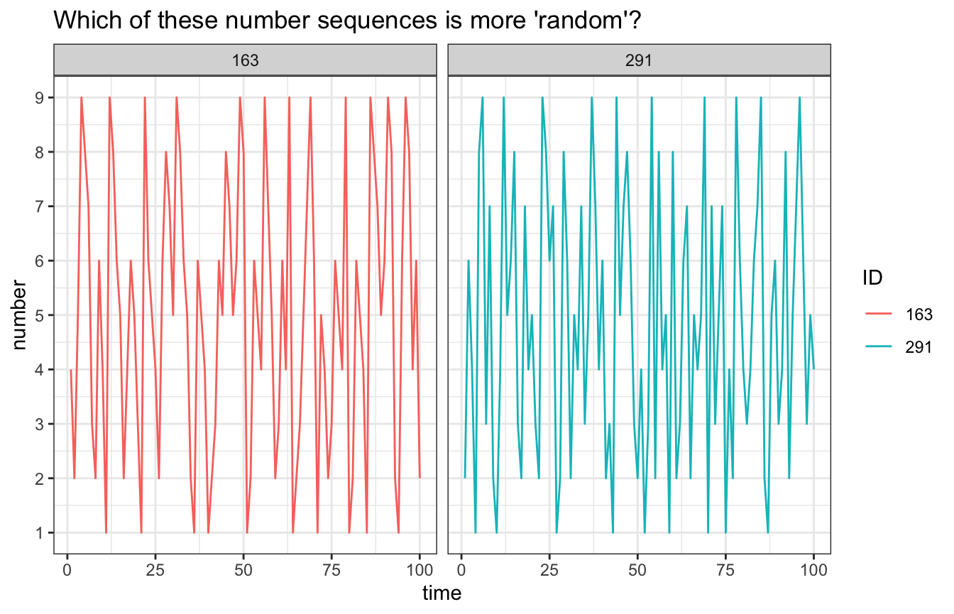
In order to answer the question in the Figure title, we’ll run a Recurrence Quantification Analysis.
The data are unordered categorical, that is, the differences between the integers are meaningless in the context of generating random number sequences. This means the RQA parameters can be set to quantify recurrences of the same value:
- Embedding lag = 1
- Embedding dimension = 1
- Radius = 0 (any number \(\leq\) 1 will do)
In the code block below the functions rp_cl(), rp(), and rp_plot() are used to perform RQA on 2 participants in the dataset.
# Run the RQA analysis
y_1  <- RNG$number[RNG$ID==163]
y_2 <-  RNG$number[RNG$ID==291]
crqa_1 <- rp_cl(y1 = y_1, emDim  = 1, emLag = 1, emRad= 1)
>
> ~~~o~~o~~casnet~~o~~o~~~
>
> Performing auto-RQA
>
> ...using sequential processing...
>
|
| | 0%
|
|o~oo~oo~oo~oo~oo~oo~oo~oo~oo~oo~oo~oo~oo~oo~oo~oo~oo~oo~oo~oo~o| 100%
>
> Completed in:
> user system elapsed
> 0.015 0.019 0.097
>
> ~~~o~~o~~casnet~~o~~o~~~>
> ~~~o~~o~~casnet~~o~~o~~~
>
> Performing auto-RQA
>
> ...using sequential processing...
>
|
| | 0%
|
|o~oo~oo~oo~oo~oo~oo~oo~oo~oo~oo~oo~oo~oo~oo~oo~oo~oo~oo~oo~oo~o| 100%
>
> Completed in:
> user system elapsed
> 0.008 0.003 0.014
>
> ~~~o~~o~~casnet~~o~~o~~~## Plot the recurrence matrix
# Get the recurrence matrix
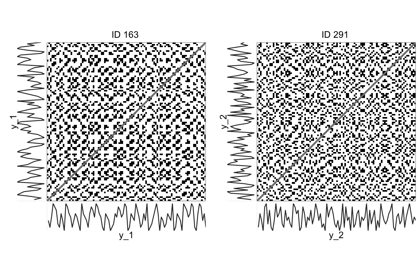
rp_1 <- rp(y1=y_1, y2=y_1, emDim = 1, emLag = 1, emRad = 1)
rp_2 <- rp(y1=y_2, y2=y_2, emDim = 1, emLag = 1, emRad = 1)
# Get the plots
g_1 <- rp_plot(rp_1, plotDimensions = TRUE, returnOnlyObject = TRUE, title = "ID 163")
g_2 <- rp_plot(rp_2, plotDimensions = TRUE, returnOnlyObject = TRUE, title = "ID 291")Below the data and plots are rearranged for ease of comparison.
>                                   subj163                          subj291
> .id      window: 1 | start: 1 | stop: 100 window: 1 | start: 1 | stop: 100
> RR                               0.114343                         0.105051
> DET                              0.399293                         0.184615
> DET.RR                            3.49205                           1.7574
> LAM                                     0                                0
> LAM.DET                                 0                                0
> L_max                                   6                                3
> L                                 2.40426                          2.04255
> L_entr                           0.837053                         0.175975
> DIV                              0.166667                         0.333333
> V_max                                   1                                1
> TT                                      0                                0
> V_entr                                  0                                0
> T1                                8.45303                          9.41424
> T2                                8.45303                          9.41424
> W_max                                  36                               31
> W_mean                            6.87014                          7.67115
> W_entr                            2.44169                          2.60211
> W_prob                                  4                                8
> F_min                           0.0277778                        0.0322581
> emDim                                   1                                1
> emLag                                   1                                1
> emRad                                   1                                1
> DLmin                                   2                                2
> VLmin                                   2                                2
> distNorm                        EUCLIDEAN                        EUCLIDEAN
The sequence generated by participant 163 has a higher DETerminism (DET = .40) than the sequence by particpant 291 (DET = .19). The ratio of points on a diagonal line to the total number of recurrent point also quantifies this difference (DET_RR). Also interesting to note, both participants have a LAMinarity score of 0. This implies they avoided to produce patterns in which the exact same numbers were repeated in succession. This is a tell-tale sign of the non-random origins of these sequences.
Hypothesis testing using constrained data realisations
A simple strategy to get some more certainty about the differences between the two sequences is to randomise the observed series, thus removing any temporal correlations that might give rise to recurring patterns in the sequences and re-run the RQA. If the repeated patterns generated by participant 163 are non-random one would expect the DETerminism to drop. If they do not drop this could indicate some random autoregressive process is causing apparent deterministic temporal patterns.
# Reproduce the same randomisation
set.seed(123456789)

# Randomise the number sequences
y_1rnd <- y_1[sample(1:NROW(y_1),size = NROW(y_1))]
y_2rnd <- y_2[sample(1:NROW(y_2),size = NROW(y_2))]

# Calculate RQA measures
crqa_1rnd <- rp_cl(y1 = y_1rnd, emDim  = 1, emLag = 1, emRad= 1)
>
> ~~~o~~o~~casnet~~o~~o~~~
>
> Performing auto-RQA
>
> ...using sequential processing...
>
|
| | 0%
|
|o~oo~oo~oo~oo~oo~oo~oo~oo~oo~oo~oo~oo~oo~oo~oo~oo~oo~oo~oo~oo~o| 100%
>
> Completed in:
> user system elapsed
> 0.009 0.002 0.013
>
> ~~~o~~o~~casnet~~o~~o~~~>
> ~~~o~~o~~casnet~~o~~o~~~
>
> Performing auto-RQA
>
> ...using sequential processing...
>
|
| | 0%
|
|o~oo~oo~oo~oo~oo~oo~oo~oo~oo~oo~oo~oo~oo~oo~oo~oo~oo~oo~oo~oo~o| 100%
>
> Completed in:
> user system elapsed
> 0.010 0.003 0.013
>
> ~~~o~~o~~casnet~~o~~o~~~# Create the recurrence matrix
rp_1 <- rp(y1=y_1rnd, y2=y_1rnd, emDim = 1, emLag = 1,emRad = 1)
rp_2 <- rp(y1=y_2rnd, y2=y_2rnd, emDim = 1, emLag = 1,emRad = 1)
# Get the RPs
g_1rnd <- rp_plot(rp_1, plotDimensions = TRUE, returnOnlyObject = TRUE, title = "ID 163 shuffled")
g_2rnd <- rp_plot(rp_2, plotDimensions = TRUE, returnOnlyObject = TRUE, title = "ID 291 shuffled")
# Display recurrence plots
cowplot::plot_grid(g_1rnd, g_2rnd, align = "h")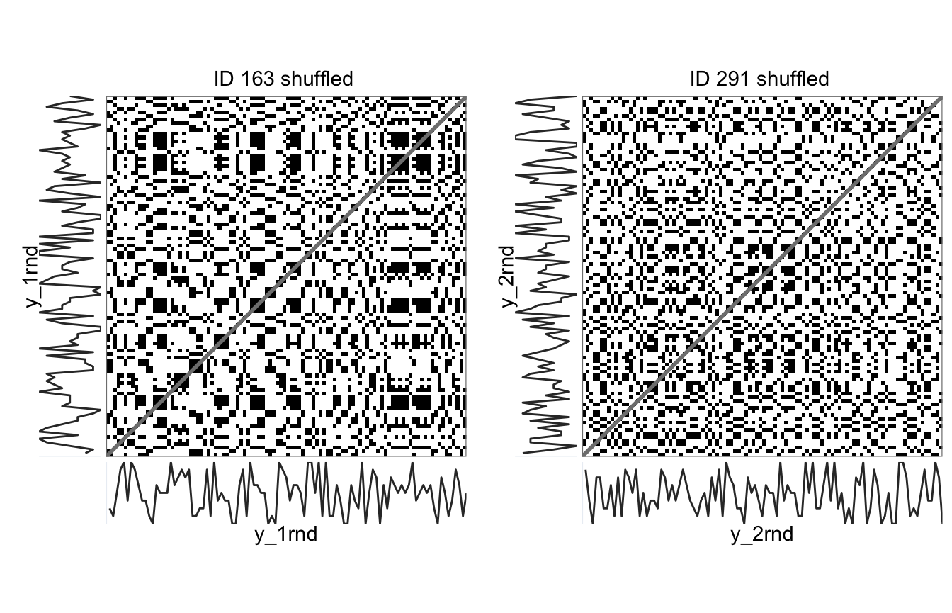
>                                   subj163                       subj163rnd
> .id      window: 1 | start: 1 | stop: 100 window: 1 | start: 1 | stop: 100
> RR                               0.114343                         0.114343
> DET                              0.399293                         0.212014
> DET.RR                            3.49205                          1.85419
> LAM                                     0                         0.241166
> LAM.DET                                 0                           1.1375
> L_max                                   6                                4
> L                                 2.40426                          2.18182
> L_entr                           0.837053                         0.496537
> DIV                              0.166667                             0.25
> V_max                                   1                                3
> TT                                      0                              2.1
> V_entr                                  0                         0.325083
> T1                                8.45303                          8.33593
> T2                                8.45303                          9.76835
> W_max                                  36                               42
> W_mean                            6.87014                          8.03838
> W_entr                            2.44169                          2.73334
> W_prob                                  4                                1
> F_min                           0.0277778                        0.0238095
> emDim                                   1                                1
> emLag                                   1                                1
> emRad                                   1                                1
> DLmin                                   2                                2
> VLmin                                   2                                2
> distNorm EUCLIDEAN EUCLIDEAN> subj291 subj291rnd
> .id window: 1 | start: 1 | stop: 100 window: 1 | start: 1 | stop: 100
> RR 0.105051 0.105051
> DET 0.184615 0.192308
> DET.RR 1.7574 1.83062
> LAM 0 0.207692
> LAM.DET 0 1.08
> L_max 3 4
> L 2.04255 2.08333
> L_entr 0.175975 0.273574
> DIV 0.333333 0.25
> V_max 1 2
> TT 0 2
> V_entr 0 0
> T1 9.41424 8.79314
> T2 9.41424 10.0049
> W_max 31 42
> W_mean 7.67115 8.16154
> W_entr 2.60211 2.77721
> W_prob 8 3
> F_min 0.0322581 0.0238095
> emDim 1 1
> emLag 1 1
> emRad 1 1
> DLmin 2 2
> VLmin 2 2
> distNorm EUCLIDEAN EUCLIDEANNote that the number of recurrent points (RR) does not change whe we shuffle the data. What changes is the number of recurrent points that form line structures in the recurrence plot. Randomising the number sequences causes vertical line structures to appear in the recurrence plot (LAM, V_max, V_entr, TT), this is what we would expect if the data generating process were indeed a random process. Having no such structures means there were hardly any sequences consisting of repetitions of the same number. Participants may have adopted a strategy to avoid such sequences because they erroneously believed this to be a feature of non-random sequences.
A permutation test with surrogate time series
In order to get an idea about the meanignfulness of these differences, we can construct a surrogate data test for each participant. If we want a one-sided test with \(\alpha=.05\), the formula for the number of constrained realisations \(M\) we minimally need is: \[M = \frac{1}{\alpha}-1 = 19\]. Add the observed value and we have a sample size of \(N = 20\). For a two sided test we would use \[M = \frac{2}{\alpha}-1 = 39\].
Of course, if there are no computational constraints on generating surrogate time series, we can go much higher, If we want \(N = 100\), the test will be an evaluation of \(H_{0}\) at \(\alpha = .01\).
- Create
99realisations that reflect a test of the hypothesis \(H_{0}: X_i \sim \mathcal{U(1,9)}\) at \(\alpha = .01\). - Calculate the measure of interest, e.g.
DET - If the observed
DETvalue is at the extremes of the distribution of values representing \(H_{0}\), the observed value was probably not generated by drawing from a discrete uniform distribution with finite elements1through9.
Use function plorSUR_hist() to get a p-value and plot the distributions. The red dots indicate the observed values.
# Get point estimates for p-values based on rank of observation (discrete distribution)
#   99 = (1 / alpha) - 1
# 99+1 = (1 / alpha)
alpha = 1/100

p_1 <- plotSUR_hist(surrogateValues = crqa_1rnd_sur$DET, observedValue = crqa_1$DET, measureName = "DET", doPlot = FALSE)
p_2 <- plotSUR_hist(surrogateValues = crqa_2rnd_sur$DET, observedValue = crqa_2$DET, measureName = "DET", doPlot = FALSE)

cowplot::plot_grid(p_1$surrogates_plot, p_2$surrogates_plot, labels = c("ID 163","ID 291"), ncol = 1)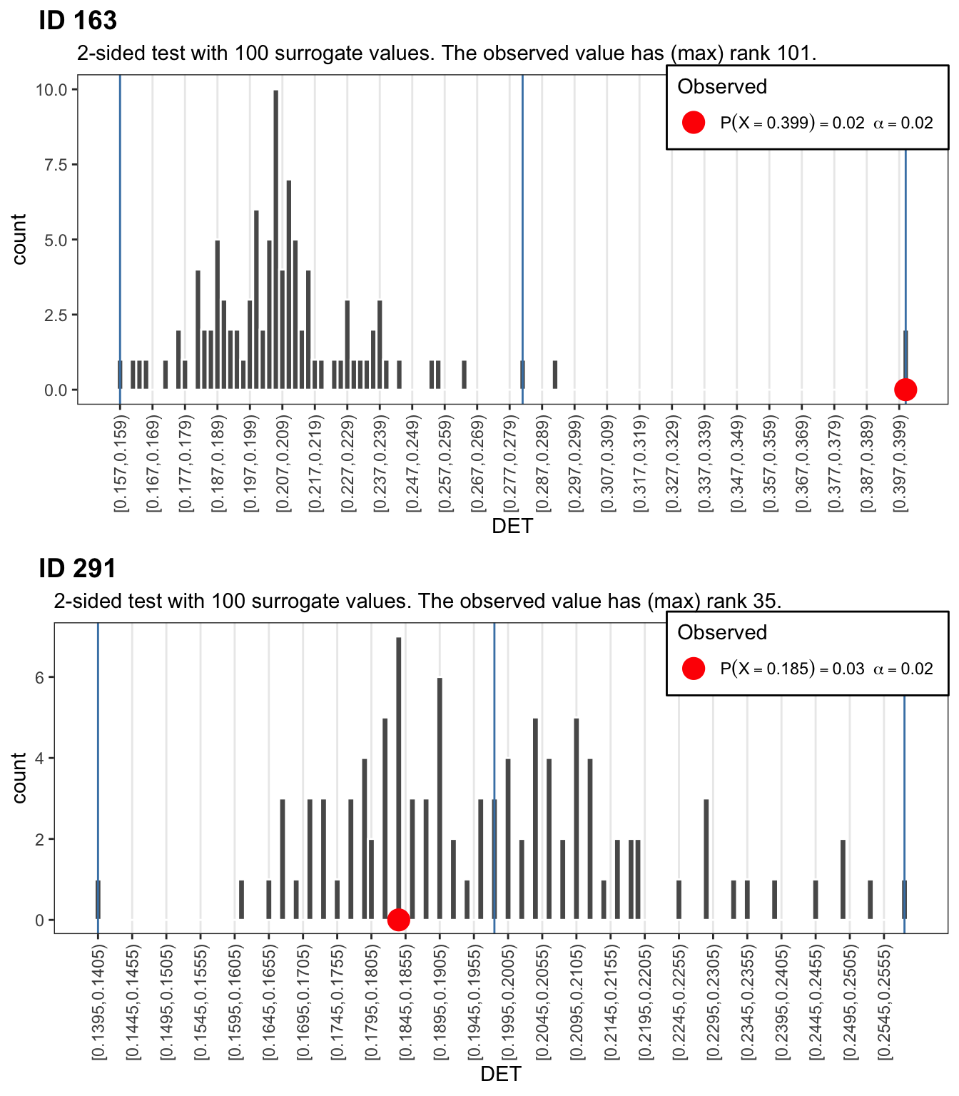
To get the full picture, let’s look at those missing repetitions of the same numbers.
# Get point estimates for p-values based on rank of observation (discrete distribution)
#   99 = (1 / alpha) - 1
# 99+1 = (1 / alpha)
alpha = 1/100

p_1 <- plotSUR_hist(surrogateValues = crqa_1rnd_sur$LAM, observedValue = crqa_1$LAM, measureName = "LAM", doPlot = FALSE)
p_2 <- plotSUR_hist(surrogateValues = crqa_2rnd_sur$LAM, observedValue = crqa_2$LAM, measureName = "LAM", doPlot = FALSE)

cowplot::plot_grid(p_1$surrogates_plot, p_2$surrogates_plot, labels = c("ID 163","ID 291"), ncol = 1)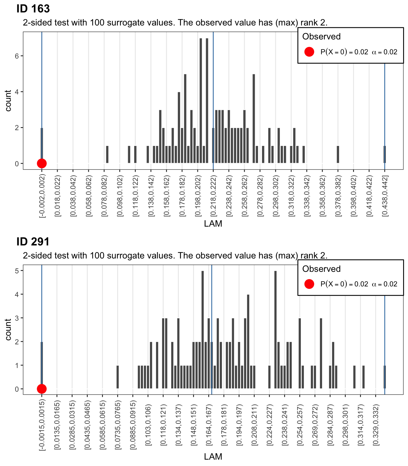
If we were naive to the orgin of these number sequences, the results for LAMinarity should make us doubt that they represent indendent draws from a discrete uniform distribution of the type \(X \sim \mathcal{U}(1,9)\). If we had to decide which sequence was more, or, less random, then based on the DETerminism result, we would conclude that participant 163 produced a sequence that is less random than participant 291, the observed value of the former is at the right extreme of a distribution of DET values calculated from 99 realisations of the data constrained by \(H_0\).
References
Oomens, W., Maes, J. H. R., Hasselman, F., & Egger, J. I. M. (2015). A time series approach to random number generation: Using recurrence quantification analysis to capture executive behavior. Frontiers in Human Neuroscience, 9, 319. https://doi.org/10.3389/fnhum.2015.00319